Overview of GSEA

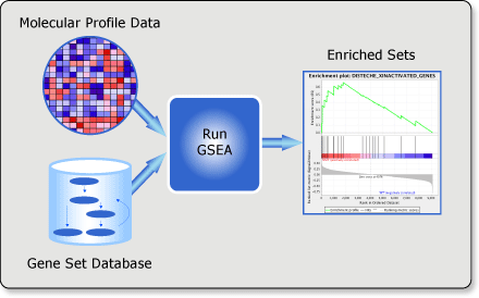
Gene set enrichment analysis (gsea) is a computational method that determines whether an a priori defined set of genes shows statistically significant, concordant differences between two biological states (e.g. phenotypes).

Input files preparation

Fast preparation

Normally we would have gene expression matrix like the file listed below:

#test.a
gene	kdctcf_1	kdctcf_2	kdctcf_3	ctl_1	ctl_2	ctl_3
a	1	2	3	4	5	6
b	1	2	3	4	5	6
c	1	2	3	4	5	6
d	1	2	3	4	5	6

#test.b
gene	kdctcf	kdctcf	kdctcf	ctl	ctl	ctl
a	1	2	3	4	5	6
b	1	2	3	4	5	6
c	1	2	3	4	5	6
d	1	2	3	4	5	6

The program transfernormalexprmatrixforgsea.py will help to transfer expression matrix to generate gct and cls file for gsea usages.

Run this script using sample data as showed below (Please refer to the program for deatiled description of input and output files.):

#transfer test.a
transfernormalexprmatrixforgsea.py -i test.a
#transfer test.b
transfernormalexprmatrixforgsea.py -i test.b -u 0
#<-u 0> indicates there are duplicates in sample names

Both commands creat same output (test.a.gct, test.a.cls, test.b.gct, test.b.cls), here only lists the first two of them:

test.a.gct

#1.2
4	6
gene	description	kdctcf_1	kdctcf_2	kdctcf_3	ctl_1	ctl_2	ctl_3
a	a	1	2	3	4	5	6
b	b	1	2	3	4	5	6
c	c	1	2	3	4	5	6
d	d	1	2	3	4	5	6

test.a.cls

6 2 1
# kdctcf ctl
kdctcf kdctcf kdctcf ctl ctl ctl

For huamn and mouse dataset, gmt files can be downloaded from gsea and enrichmentmap.

Now, we have got all required files for GSEA analysis.

Detailed description for each file

• gct fileformat

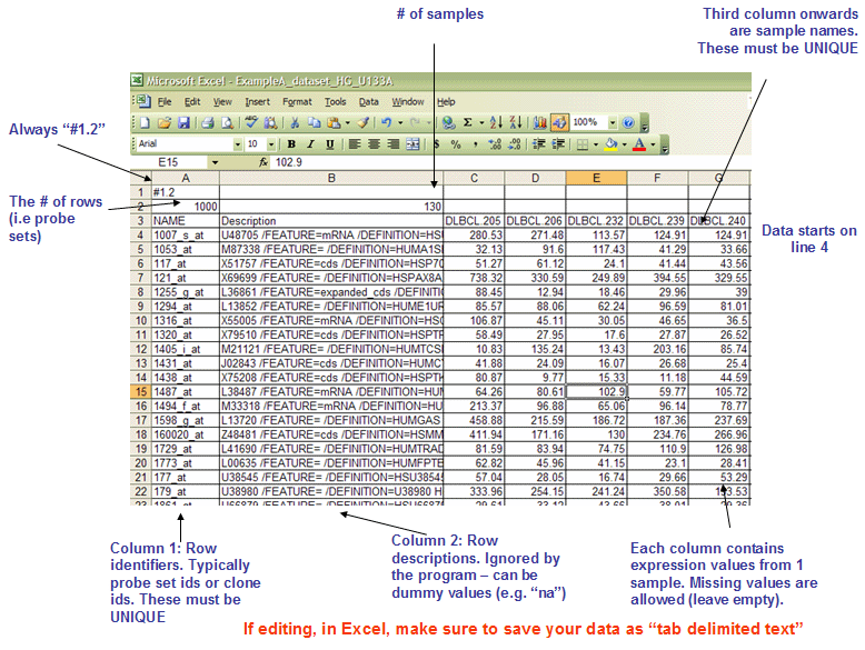
* The first line should always be `#1.2`.
* The second line contains tow columns, `(# of genes)<tab>(# of samples)`.
* The first two columns of data lines are `gene name` (should be unique) and `gene description` (which will not be used in gsea, usually it can be the same as gene name).

• cls format

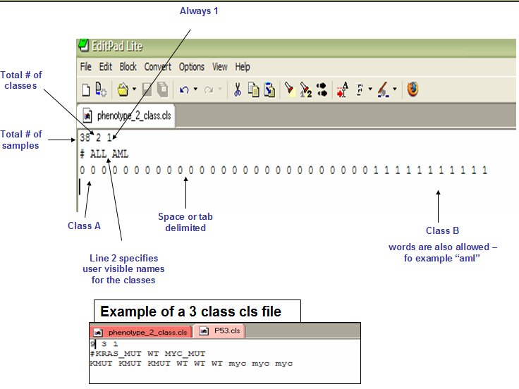
* The first line contains `(# of damples)<space>(# of classes)<space>1`.
* The second line contains `#<space>(class 0 name)<space>(class 1 name)...`.
* The third line contains `(class1-samp1)<space>(class1-samp2)<space>(class2-samp1)...`.

• gmt format

The GMT file format is a tab delimited file format that describes gene sets. In the GMT format, each row represents a gene set; in the GMX format, each column represents a gene set. The GMT file format is organized as follows:

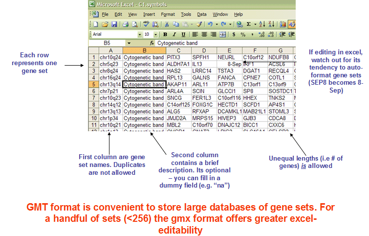
Each gene set is described by a name, a description, and the genes in the gene set. GSEA uses the description field to determine what hyperlink to provide in the report for the gene set description: if the description is “na”, GSEA provides a link to the named gene set in MSigDB; if the description is a URL, GSEA provides a link to that URL.

Since I can directly download gmt files from gsea and enrichmentmap, I have not tried to generate gmt files.

Run gsea

Below steps are borrowed from http://www.baderlab.org/Software/EnrichmentMap/Tutorial. There is also sample data in their web sites for testing this tutorial.

• GO to GSEA website - http://www.broadinstitute.org/gsea/.
• Click on Downloads in the page header.
  • From the javaGSEA Desktop Application right click on Launch with 1 Gb memory.
  • Click on “Save Target as…” and save shortcut to your desktop or your folder of choice so you can launch GSEA for your analysis without having to navigate to it through your web browser.
• Double click on GSEA icon you created.
  • Specially, runing javaws gsea.jnlp to start GSEA in linux.
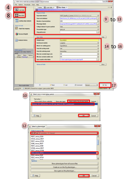
• Click on Load data in left panel.
• Click on Browse for files in newly opened Load data panel.
• Navigate to directory where you stored tutorial test set files. Select all raw expression (.gct) file, sample class file(.cls) and gene set (.gmt) file. Click on Open.
• Wait until confirmation box appears indicating that all files loaded successfully. Click on Ok.
• Click on Run GSEA in left panel.
• Select the Expression dataset:
  • Click on the arrow next to the Expression dataset text box.
  • Select the expression set you wish to run the analysis on (MCF7_ExprMx_v2_names.gct).
• Select the Gene Set Database:
  • Click on … next to the text box of Gene Set Database.
  • Click on Gene Matrix (local gmx/gmt) tab.
  • Select gmt file Human_GO_AllPathways_no_GO_iea_April_15_2013_symbo.gmt and click on Ok.
• Select the Phenotype labels file
  • Click on … next to the text box of Phenotype labels.
  • Make sure Select source file is set to ES_NT.cls.
  • Select ES12_versus_NT12 and click on Ok.
• Click on the down arrow next to the text box for Collapse dataset to gene symbols, select false.
• Click on the down arrow next to the text box for Permutation type, select gene_set.
• Click on Show next to Basic fields.
• Click in text box next to Analysis name and rename (example:estrogen_treatment_12hr_gsea_enrichment_results).
• Click on … next to “Save results” in this folder text box. Navigate to the folder where you wish to save the results (preferably the same directory where all the input files have been saved).
• Click on Run in the bottom right corner.
• Wait untial the status in left panel is success. The output will be saved in input folder.

GSEA result interpretation

The primary result of the gene set enrichment analysis is the enrichment score (ES), which reflects the degree to which a gene set is overrepresented at the top or bottom of a ranked list of genes. GSEA calculates the ES by walking down the ranked list of genes, increasing a running-sum statistic when a gene is in the gene set and decreasing it when it is not. The magnitude of the increment depends on the correlation of the gene with the phenotype. The ES is the maximum deviation from zero encountered in walking the list. A positive ES indicates gene set enrichment at the top of the ranked list; a negative ES indicates gene set enrichment at the bottom of the ranked list.

In the analysis results, the enrichment plot provides a graphical view of the enrichment score for a gene set:

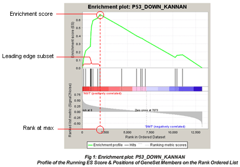
The red fonts are “MUT(positively correlated)” and blue fonts are “WT(negatively correlated)”. The picture indicates enrichment of “P53_DOWN_KANNAN” in MUT versus WT cells.

• The top portion of the plot shows the running ES for the gene set as the analysis walks down the ranked list. The score at the peak of the plot (the score furthest from 0.0) is the ES for the gene set. Gene sets with a distinct peak at the beginning (such as the one shown here) or end of the ranked list are generally the most interesting.

• The middle portion of the plot shows where the members of the gene set appear in the ranked list of genes.

The leading edge subset of a gene set is the subset of members that contribute most to the ES. For a positive ES (such as the one shown here), the leading edge subset is the set of members that appear in the ranked list prior to the peak score. For a negative ES, it is the set of members that appear subsequent to the peak score.

• The bottom portion of the plot shows the value of the ranking metric as you move down the list of ranked genes. The ranking metric measures a gene’s correlation with a phenotype. The value of the ranking metric goes from positive to negative as you move down the ranked list. A positive value indicates correlation with the first phenotype and a negative value indicates correlation with the second phenotype. For continuous phenotypes (time series or gene of interest), a positive value indicates correlation with the phenotype profile and a negative value indicates no correlation or inverse correlation with the profile.

The normalized enrichment score (NES) is the primary statistic for examining gene set enrichment results. By normalizing the enrichment score, GSEA accounts for differences in gene set size and in correlations between gene sets and the expression dataset; therefore, the normalized enrichment scores (NES) can be used to compare analysis results across gene sets. GSEA determines NES as follows:

NES = actual ES / mean(ESs against all permutations of the dataset)

NES is based on the gene set enrichment scores for all dataset permutations; therefore, changing the permutation method, the number of permutations, or the size of the expression dataset affects the NES. As an example, consider two analyses: (1) you analyze an expression dataset, GSEA generates a ranked list and analyzes that ranked list; (2) you use GSEAPreranked to analyze the ranked list generated by the first analysis. If you use the same parameter settings, your enrichment scores are identical; however, the normalized enrichment scores reflect the very different datasets (the expression dataset versus the ranked list of genes) used for the permutations.

The false discovery rate (FDR) is the estimated probability that a gene set with a given NES represents a false positive finding. For example, an FDR of 25% indicates that the result is likely to be valid 3 out of 4 times. The GSEA analysis report highlights enrichment gene sets with an FDR of less than 25% as those most likely to generate interesting hypotheses and drive further research, but provides analysis results for all analyzed gene sets. In general, given the lack of coherence in most expression datasets and the relatively small number of gene sets being analyzed, an FDR cutoff of 25% is appropriate. However, if you have a small number of samples and use gene_set permutation (rather than phenotype permutation) for your analysis, you are using a less stringent assessment of significance and would then want to use a more stringent FDR cutoff, such as 5%.

The FDR is a ratio of two distributions: (1) the actual enrichment score versus the enrichment scores for all gene sets against all permutations of the dataset and (2) the actual enrichment score versus the enrichment scores of all gene sets against the actual dataset. For example, if you analyze four gene sets and run 1000 permutations, the first distribution contains 4000 data points and the second contains 4. For an example of what the enrichment score for a permutation of the dataset might look like, consider the two enrichment plots shown below. The plot on the left shows actual enrichment results for the P53HYPOSIAPATHWAY gene set against the P53 dataset. The plot on the right shows enrichment results for that gene set against a phenotype permutation of the dataset (that is, when phenotype labels are randomly assigned to the samples).

Reference

• http://www.broadinstitute.org/cancer/software/gsea/wiki/index.php/Data_formats
• http://www.broadinstitute.org/gsea/downloads.jsp
• http://www.baderlab.org/Software/EnrichmentMap/Tutorial
• http://www.broadinstitute.org/gsea/doc/GSEAUserGuideFrame.html