这篇文章用于记录学习贝叶斯定理及其应用过程中的记录,希望由浅及深的提供 一份自我学习教程。
引子
-
概率的定义:概率是一个0-1之间的数,代表了我们对某个事实或预测的相信程度。
-
条件概率: 指基于某种背景信息的概率值。
-
联合概率:指2个或多个事件同时发生的概率。
-
事件独立性:一个事件的发生不影响其他事件即为事件的独行性。
-
概率的数学表示:事件A发生的概率写作 P(A), 事件B发生的概率写作 P(B), 给定事件A后事件B发生的概率 P(B|A), 事件A和B同时发生的概率P(A and B)。
-
事件的独立性用数学公式表示为:P(B|A) = P(B), P(A|B) = P(A) A事件是否发生对B事件的发生没有影响,反之亦然, 即表明A事件与B事件独立。
-
联合概率:P(A and B) = P(A) * P(B) 当事件A和B独立时,即 P(B|A) = P(B), P(A|B) = P(A) 时。
若事件A和事件B不一定相互独立呢?更通用的法则是:
P(A and B) = P(A) * P(B|A) P(A and B) = P(B) * P(A|B) -
我们举个例子:假设有袋圆球,罐1中有30个黑球和10个白球,罐2中黑球和白球各20个。某人随机的从一个罐子中取出一粒球,发现是黑球,问这个黑球从罐1中取出的概率有多大?
这个问题怎么解答呢?
问题是:黑球从罐1中取出的概率多大;这句话包含了2个事件,
黑球和罐1.假如我们知道取得黑球的概率P(黑球)和给定黑球后球是从罐1取得的概率 P(罐1|黑球)(这个是我们要计算的,假设个变量标记下就好), 我们可以计算出联合概率: P(黑球 and 罐1) = P(黑球)*P(罐1|黑球)
另外我们也可以先选择罐1,然后再取出黑球,这样联合概率就是: P(黑球 and 罐1) = P(罐1)*P(黑球|罐1)
综合以上2个公式,我们就可以得到:
P(黑球)*P(罐1|黑球) = P(罐1)*P(黑球|罐1)

P(罐1|黑球) = P(罐1)*P(黑球|罐1) / P(黑球)

= P(罐1)*P(黑球|罐1) / (P(罐1)*P(黑球|罐1)+P(罐2)*P(黑球|罐2))

= 0.5 * 0.75 / (0.5 * 0.75 + 0.5 * 0.5)

= 0.6
注:这是一个简单的例子作为引子,是一个非常规解法。 例子中的P(黑球)可以比较容易计算,所 以我们只需要一步就可以算出黑球从罐1中取出的概率有多大。
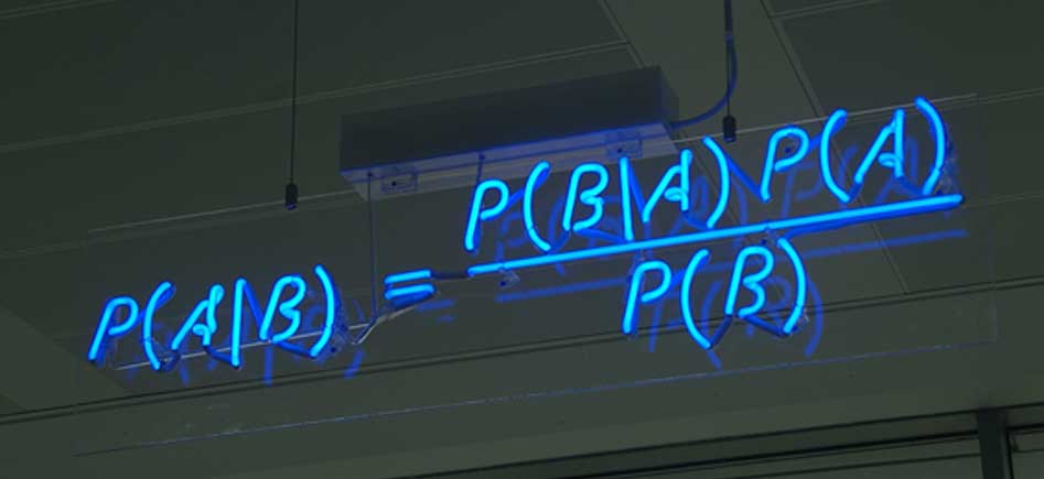
贝叶斯定理
-
基于联合概率和条件概率的贝叶斯定理推导
对于任意两个事件A和B,P(A and B) = P(B and A);
P(A and B) = P(A) * P(B|A)

P(B and A) = P(B) * P(A|B)

P(A|B) = P(A)*P(B|A)/P(B)

P(B|A) = P(B)*P(A|B)/P(A)
在有了这两个转换之后,我们就可以用已知的或者容易观察的数据来计算未知 的,不容易观察到的部分。
-
贝叶斯定理解释: 贝叶斯定理反应的是随着数据的更新而得以矫正的概率值。
设定H代表我们的假说,D代表观测数据,贝叶斯定理可以写做
P(H|D) = P(H)*P(D|H) / P(D)-
P(H): 先验概率,反应的是主观对假说H的认可度, 反应的是获得观察数据之前的认识。
-
P(H|D): 后验概率,在分析了观察数据之后对假说H的新的认识, 反应的是根据新的事实对H发生的概率的更新。
-
P(D|H): 似然值,在假设成立的条件下,可以获得这组观察数据的概率。
-
P(D): 在任何假设条件下,获取到这组观察数据的概率。通常难以计算。
-
在这个公式中,观察数据是已经获得的。假说也是容易提出的。 在假说成立的条件下,数据的模式是可以估计的。 三个变量,这儿解决了2个。
-
通常情况下,为了规避对P(D)的计算,我们会穷举出所有独立的假设 (在这些假设中,最多有一个是真的,也至少有一个是真的), 分别计算P(H1|D), P(H2|D), P(H3|D)…, 根据所有这些概率的和为1进行归一化,获得各个假设在给定的当前数据模 式下成立的概率。
-
About normalizing constant, we simplify things by specifying a set of hypotheses that are mutually exclusive and collectively exhaustive.
-
在遇到问题时,D和H也并不总会很清晰,既需要我们多梳理问题, 明确哪个观察数据是有意义的,更需要我们熟悉较多的例子, 加深对贝叶斯定理应用的理解。
-
-
Explanation of Bayes’ rule
Bayesian inference derives the posterior probability as a consequence of two antecedents, a prior probability and a “likelihood function” derived from a statistical model for the observed data. Bayesian inference computes the posterior probability according to Bayes’ theorem:
P(H|E) = P(H)*P(E|H) / P(E)
where
|denotes a conditional probability (so that (A|B)} means A given B).Hstands for any hypothesis whose probability may be affected by data (called evidence below). Often there are competing hypotheses, and the task is to determine which is the most probable.- the evidence
Ecorresponds to new data that were not used in computing the prior probability. P(H), the prior probability, is the estimate of the probability of the hypothesisHbefore the dataE, the current evidence, is observed.P(H|E)the posterior probability, is the probability ofHgivenE, i.e., afterEis observed. This is what we want to know: the probability of a hypothesis given the observed evidence.P(E|H)is the probability of observingEgivenH. As a function ofEwithHfixed, this is the likelihood –it indicates the compatibility of the evidence with the given hypothesis. The likelihood function is a function of the evidence,E, while the posterior probability is a function of the hypothesis,H.P(E)is sometimes termed the marginal likelihood or “model evidence”. This factor is the same for all possible hypotheses being considered (as is evident from the fact that the hypothesisHdoes not appear anywhere in the symbol, unlike for all the other factors), so this factor does not enter into determining the relative probabilities of different hypotheses.
For different values of
H, only the factorsP(H)andP(E|H), both in the numerator, affect the value ofP(H|E)-the posterior probability of a hypothesis is proportional to its prior probability (its inherent likeliness) and the newly acquired likelihood (its compatibility with the new observed evidence).
贝叶斯定理的现实意义
贝叶斯方法来源于托马斯·贝叶斯s生前为解决一个“逆概”问题而写的文章。 在贝叶斯之前,“正向概率”已经能够计算,如“假设封闭袋子里有N个白球, M个黑球,随机摸一个出来是黑球的概率有多大”。 而一个自然而然的反向思考是:如果事先不知道袋子里面黑白球的比例, 随机取出一个(或多个)球,观察取出的球的颜色, 是否就可以推测袋子里黑白球的比例?
这正如我们日常所观察到的都是表面的结果,很难看到事务后面的本质, 如上述例子中封闭袋子里黑白球的比例。因此我们需要根据我们的观察, 提出一个猜测或假设,然后评估这个假设发生的概率。如算出不同猜测的可能性 大小,即后验概率。对于连续的猜测空间,则是计算猜测的概率密度函数; 最后得到最靠谱的猜测。
概括来讲,贝叶斯方法是一个分而治之的思想,把难以计算的概率用先验知识和 似然值估算出来。也反映了我们随着观察的不管深入,对之前的认识的不断更新。
P(H|D) = P(H)*P(D|H)/P(D)
最优贝叶斯推理
贝叶斯推理分为两个过程;第一步是根据观测数据穷举出全部独立的模型,也叫假设; 第二步是使用模型推测未知现象发生的概率。这时我们不是选择最靠谱的模型, 而是把全部模型对未知的预测加权平均起来(权重值就是模型相应的概率)。
贝叶斯定理应用案例
判断男女
一所学校,男生60%,女生40%。男生总是穿长裤,女生则一半穿长裤, 一半穿裙子。假设高度近视的你未带眼镜走在校园中, 发现迎面走来一个穿裤子的学生,但未分辨出男女, 那么推断这个是男生的概率多大?
D是:穿裤子的学生。
H是:A:这个学生是男生;B:这个学生是女生
待求:P(A|D) = P(男生|长裤)
表格表示
| Prior | Likelihood | Posterior | ||
|---|---|---|---|---|
| P(H) | P(D|H) | P(H)*P(D|H) | P(H|D) | |
| A | 0.6 | 1 | 0.6 | 3/4 |
| B | 0.4 | 0.5 | 0.2 | 1/4 |
M&M豆问题
公司在不同年份生产的M&M豆包含的不同颜色的豆的比例不同, 1994年产的M&M豆包装中,棕色30%,黄色20%,红色20%,绿色10%,橙色10%, 茶色10%;1996年产的M&M豆包装中,棕色13%,黄色14%,红色13%,绿色20%, 橙色16%,蓝色24%。假设手中有两粒M&M豆,分别是橙色和绿色, 一个来自1994年包装,一个来自1996年包装,求算橙色来源于1994年包装的概率?
解题思路:
-
观察到的数据 D:橙色球和绿色球个来自不同包装
-
完全穷举独立假设
- 假设A:橙色来源于94,绿色来源于96
- 假设B:橙色来源于96,绿色来源于94
-
假设A和假设B发生的概率是一样的,都为0.5.
-
似然值的计算
- 假设A:P(橙色|94)*P(绿色|96) = 0.1 * 0.2 = 0.02
- 假设B:P(橙色|96)*P(绿色|94) = 0.16 * 0.1 = 0.016
为了计算方便,似然值可以乘以任意一个因子,不影响结果。
- 假设A:P(橙色|94)*P(绿色|96) = 0.1 * 0.2 * 100 = 20
- 假设B:P(橙色|96)*P(绿色|94) = 0.16 * 0.1 * 100 = 16
为了计算方便,似然值可以乘以任意一个因子,不影响结果。
-
后验概率
- P(A|D) ∝ 0.05 * 20 = 10
- P(B|D) ∝ 0.05 * 16 = 8
-
Normalize概率:P(A|D) = 10/18 = 5/9。因为穷举了所有假设, 所以后验概率之和为1.
表格表示
| Prior | Likelihood | Posterior | ||
|---|---|---|---|---|
| P(H) | P(D|H) | P(H)*P(D|H) | P(H|D) | |
| A | 0.5 | 10 * 20 | 100 | 5/9 |
| B | 0.5 | 16 * 10 | 80 | 4/9 |
-
在提出假设时, 假设要完整穷尽,然后给每个假设指定一个代号便于描述和理清思路。
-
不明确的变量和概率值也用一个符号表示,便于列出公式。这一点我们后面还会提到。
Monty Hall问题
Suppose you’re on a game show, and you’re given the choice of three doors: Behind one door is a car; behind the others, goats. You pick a door, say No. 1, and the host, who knows what’s behind the doors, opens another door, say No. 3, which has a goat. He then says to you, “Do you want to pick door No. 2?” Is it to your advantage to switch your choice?”
有个游戏,翻译过来暂且叫“开门大吉”。Monty向你展示3个关着的门, 每个门后面都有一个奖品,其中一个是汽车,另外两个是不值钱的物品, 参与人选中一个门,如果门后面是车,则车子归参与人所有。 假设你选中了一个门A,还剩下两个门B和C。在打开你选中的门A之前, Monty会随机打开另外两个门中的一个,比如B,发现门后面没有车。 这时Monty会问你要不要坚持之前的选择A还是选择C?
-
解决这个问题最关键的地方是:D是什么?即我们观察到的数据是什么?
-
在这个问题中D是:Monty选择了门B,且门B后面没有车。
-
我们需要做的假设就是:车在门A后面或车在门C后面。
-
需要计算的概率就是:P(A|D),P(C|D),并且P(B|D)=0。
P(A|D) ∝ P(A)*P(D|A) = 1/3 * 1/2 = 1/6
P(B|D) ∝ P(B)*P(D|B) = 0
P(C|D) ∝ P(C)*P(D|C) = 1/3 * 1   = 1/3
表格表示
Prior Likelihood Posterior P(H) P(D|H) P(H)*P(D|H) P(H|D) A 1/3 1/2 * 1 1/6 1/3 B 1/3 0 0 0 C 1/3 1 1/3 2/3 - 假设车在门A的后面,Monty选择打开门B的概率是1/2, 门B后面没有车的概率是1。
- 假设车在门B的后面,Monty打开门B且后面无车的概率是0。
- 假设车在门C的后面,Monty只能选择打开门B,概率为1。
注:
- Monty打开的门是B还是C不影响最终的结果,只要Monty打开的门后面没有车,游戏就可以继续
-
三个假设很容易提出,较难发现的是我们观察到的是什么,即D是什么。
-
最简单的解释:车在门A后面的概率是1/3,不管Monty有没有打开剩下的2个门, 只要打开的门后面没有车,也不论Monty打开剩下的两个门的哪一个。 3个门后面肯定有一个有车,Monty打开一个门没有车, 那么另外一个门后面有车的概率是1-1/3=2/3。
-
题外话:
Wikipedia上有这个问题的详细描述 https://en.wikipedia.org/wiki/Monty_Hall_problem, 从不同的角度解释了这个问题,并引出了心理学研究如下:
The problem continues to attract the attention of cognitive psychologists. The typical behavior of the majority, i.e., not switching, may be explained by phenomena known in the psychological literature as: 1) the endowment effect (Kahneman et al., 1991); people tend to overvalue the winning probability of the already chosen – already “ owned” – door; 2) the status quo bias (Samuelson and Zeckhauser, 1988); people prefer to stick with the choice of door they have already made; 3) the errors of omission vs. errors of commission effect (Gilovich et al., 1995); all else considered equal, people prefer any errors they are responsible for to have occurred through ‘omission’ of taking action, rather than through having taken an explicit action that later becomes known to have been erroneous. Experimental evidence confirms that these are plausible explanations which do not depend on probability intuition (Kaivanto et al., 2014; Morone and Fiore, 2007).
老人患癌率
Suppose that an individual’s probability of having cancer, assigned according to the general prevalence of cancer, is 1%. This is known as the ‘base rate’ or prior (i.e. before being informed about the particular case at hand) probability of having cancer.
Next, suppose that the person is 65 years old. Let us assume that cancer and age are related. The probability that a person has cancer when they are 65 years old is known as the ‘current probability’, where “current” refers to the theorised situation upon finding out information about the particular case at hand.
Then, suppose that the probability of being 65 years old is 0.2%, and that the probability of a person diagnosed with cancer being 65 years old is 0.5% (a greater probability than that of being 65 years old).
Knowing this, along with the base rate, what is the probability of having cancer giving a person is 65 years old.
假设人群中每个人患癌的概率为1%。老年人(65岁)占人群比例的0.2%。 患有癌症的老年人占人群比例的0.5%。那么给定一位65岁老人,推测其患癌症的 概率是多少?
- 观察到的数据D: 65岁老人
- 假设 H:患有癌症
- P(H|D) = P(H)*P(D|H)/P(D) = 0.5 * 1 / 0.2 / 100 = 2.5%。
It may come as a surprise that even though being 65 years old increases the risk of having cancer, that person’s probability of having cancer is still fairly low. This is because the base rate of cancer (regardless of age) is low. This illustrates both the importance of base rate, as well as that it is commonly neglected. Base rate neglect leads to serious misinterpretation of statistics; therefore, special care should be taken to avoid such mistakes. Becoming familiar with Bayes’ theorem is one way to combat the natural tendency to neglect base rates.
在利用贝叶斯定理处理问题时,要注意先验概率的获取。少数情况可以随便假设 ,多数情况需要对先验概率有个模型或者好的统计资料来计算。只有在有足够多 的观察或者合适的似然值模型下,先验概率的影响才会变小。
血型罪犯问题
Two people have left traces of their own blood at the scene of a crime. A suspect, Oliver, is tested and found to have type O blood. The blood groups of the two traces are found to be of type O (a common type in the local population, having frequency 60%) and of type AB (a rare type, with frequency 1%). Do these data (the blood types found at the scene) give evidence in favour of the proposition that Oliver was one of the two people whose blood was found at the scene?
凶杀案现场留有两个人的血迹,一种为常见的O型血(人群中出现概率60%), 另一种为AB型血(人群中出现概率为1%)。一位叫Oliver的人被认定为嫌疑人, 经检测其位O型血,则请判断现场中血迹有一个来源于Oliver的概率多大?
- 首先判断D是:现场留有2人的血迹,一个是O型,一个是AB型。
- 假设是:A:血迹有一个来源于Oliver;B:血迹都不来源于Oliver
- P(A|D) ∝ P(A)*P(D|A) = P(A) * 1% = 0.01
- 在假设A成立的条件下,其中一份血迹来源于Oliver,为B型血的概率为1. 另一份血迹为A型血的概率为1%。
- P(B|D) ∝ P(B)*P(D|B) = P(B) * 2 * 60% * 1% = 0.012
- 在假设B成立的条件下,D就是任意2个人,一个是O型,另外一个是AB型的 概率是多少;这2个人任何一个都可以为O,另一个为AB,是排列问题。
-
这儿我们假设P(A)==P(B)
- 实际上这个问题关注的是似然值,即当前证据时否可以定罪。所以可以忽略P(A)和P(B)。
- 这个结论表明证据与假设一致却不一定支持假设。
吸烟与肺癌
According to the CDC, “Compared to nonsmokers, men who smoke are about 23 times more likely to develop lung cancer and women who smoke are about 13 times more likely.” If you learn that a woman has been diagnosed with lung cancer, and you know nothing else about her, what is the probability that she is a smoker?
据CDC统计,与不抽烟者相比,抽烟的男人患肺癌的几率高23倍,抽烟的女性患 肺癌的几率高13倍。现有一名女性,诊断为肺癌,请判断她抽烟的概率多大?
- 首先判断D是:女性肺癌
-
假设是:A:该女性抽烟;B:该女性不抽烟
- 假设女性中抽烟的比例是X,则不抽烟的比例为1-X。
-
假设不抽烟的人得肺癌的几率为Y,则抽烟得肺癌的几率为13Y。
- P(A|D) ∝ P(A)*P(D|A) = X * 13Y
- P(B|D) ∝ P(B)*P(D|B) = (1-X) * Y
- 概率A和概率Bnormalize之后和为1, 则P(A|D)=13X/(1+12X)
注:
- 善于假设变量,未知的变量用符号表示出来,便于梳理公式和进一步求解。
- 把一时未知的东西用简单的符号表示下,一步步列出,有助于整理思路 ,发现解决问题的方法。
西雅图下雨
You’re about to get on a plane to Seattle. You want to know if you should bring an umbrella. You call 3 random friends of yours who live there and ask each independently if it’s raining. Each of your friends has a 2/3 chance of telling you the truth and a 1/3 chance of messing with you by lying. All 3 friends tell you that “Yes” it is raining. What is the probability that it’s actually raining in Seattle?
你打算去西雅图旅游,但不确定是否会下雨。你打电话给三个在西雅图居住但彼 此不认识的朋友打电话询问下。你的每个朋友都有2/3的可能告诉你真实情况, 也有1/3的可能他们会搞砸。询问后所有的朋友都告诉你会下雨。 那么请问西雅图下雨的概率有多大?
- 首先确认观察数据 D:三人都说会下雨。
-
假设:A: 西雅图会下雨;B:西雅图不会下雨。
-
另外还需要假设一个变量:西雅图下雨的先验概率是多少,假设为X,则不下雨的概率为(1-X)。
- P(A|D) ∝ P(A)*P(D|A) = X * 2/3 * 2/3 * 2/3 = 8X/9
- P(B|D) ∝ P(B)*P(D|B) = (1-X) * 1/3 * 1/3 * 1/3 = (1-X)/9
假如X为0.5,则西雅图下雨的概率P(A|D) = 8/9。
根据1965-99年记录的气象资料显示,西雅图一年有822个小时在下雨,约占全年 的10%。即西雅图会下雨的先验概率是10%。以此计算的后验概率 P(A|D)=8/17。
另外一种基于odds的思考方法,给定西雅图下雨的先验概率为10%,则下雨与不 下雨的先验优势比 (prior odds)为1:9。每个朋友判断正确的概率为判断错误的 概率的2倍。每个朋友对下雨贡献的似然值为2。先验优势比与似然值相乘后得到 后验优势比(posterior odds)为8:9, 对应于下雨的概率是8/17。
A base rate of 10% corresponds to prior odds of 1:9. Each friend is twice as likely to tell the truth as to lie, so each friend contributes evidence in favor of rain with a likelihood ratio, or Bayes factor, of 2. Multiplying the prior odds by the likelihood ratios yields posterior odds 8:9, which corresponds to probability 8/17, or 0.47.
药物测试
Suppose a drug test is 99% sensitive and 99% specific. That is, the test will produce 99% true positive results for drug users and 99% true negative results for non-drug users. Suppose that 0.5% of people are users of the drug. If a randomly selected individual tests positive, what is the probability that he is a user?
假设一项药物测试的假阳性率(非特异性)和假阴性率(不敏感性)都是1%。 已知人群中服用过该药物的个体约占0.5%。如果随机选择一个个体检测为阳性, 那么他服药的概率是多少?
- 观察到的数据 D: 药物测试阳性
-
假设 H1:该个体服药; H2:该未个体服药
- P(H1|D) ∝ P(H1) * P(D|H1) = 0.5% * 99% = 0.495%
-
P(H2|D) ∝ P(H2) * P(D|H2) = (1-0.5%) * 1% = 0.995%
-
Normalize后,后验概率P(H1|D) = 4.95 / (4.95+9.95) = 33.2%
-
尽管这个测试的准确率比较高,但测试结果为阳性却表明个体没有服药的可能 性更大。这又一次表明基准概率(先验概率)的重要性。
-
之所以有这么一个反直觉的结果是因为未嗑药个体远多于嗑药个体。 导致了假阳性率(0.995%)远高于真阳性率(0.495%)。
-
举个例子,假如测试了1000例个体,我们期待获得995个未嗑药,5个嗑药。 995个未嗑药个体中有0.01* 995 ≈10个会出现检测结果阳性。 5个嗑药个体中有0.99 * 5 ≈5个检测结果阳性。 所以在15个阳性检测结果中,只有约33%为真阳性。
-
如果敏感性提高到100%,而特异性依然为99%,则:
- P(H1|D) ∝ P(H1) * P(D|H1) = 0.5% * 100% = 0.5%
- P(H2|D) ∝ P(H2) * P(D|H2) = (1-0.5%) * 1% = 0.995%
- P(H1|D) = 5 / (5+9.95) = 33.4%
-
如果敏感性依然为99%,而特异性提高到99.5%,则:
- P(H1|D) ∝ P(H1) * P(D|H1) = 0.5% * 99% = 0.495%
- P(H2|D) ∝ P(H2) * P(D|H2) = (1-0.5%) * 0.5% = 0.4975%
- P(H1|D) = 4.95 / (4.95+4.975) = 49.87%
- 因此提高检测的特异性才能更好的明确检测结果。
贝叶斯法则 (Bayes’ rule)
在概率论应用中,贝叶斯法则指事件A1相对于事件A2在给定另一事件之前和之后 的比值比(odds ratio)。先验比值比(prior odds ratio)是事件之间先验概率的比值。 后验比值比(posterior odds ratio)是在给定条件事件之后的后验概率的比值。 后验比值比正相关于先验比值比乘以似然值(likelihood ratio, 又称Bayes factor)。
# O: odds ratio
# ^: likelihood
# P: probability

O(A1:A2|B) = ^(A1:A2|B) * O(A1:A2)

^(A1:A2|B) = P(B|A1) / P(B|A2)

O(A1:A2) = P(A1) / P(A2)

O(A1:A2|B) = P(A1|B) / P(A2|B)
假设一项药物测试的假阳性率(非特异性)和假阴性率(不敏感性)都是1%。 已知人群中服用过该药物的个体约占0.5%。如果随机选择一个个体检测为阳性, 那么他服药的概率是多少?
如果用贝叶斯法则的比值比来表示:
- 个体嗑药的prior odds: 0.5:99.5 = 1:199
- 个体测试为阳性的Bayes factor: 99:1
- 个体嗑药的posterior odds: 1* 99 : 199 * 1
Code representation
Here lists all code for bayes learning in ipython notbook format.
- Scan version of handwritting
- Think bayes - Chapter 2
- Think bayes - Chapter 3
- Think bayes - Chapter 4